Tutorials
Having trouble knowing where to start? These tutorials cover key functionality in bitesized chuncks. You can jump to any specific tutorial in the navigation bar or go through them all! As functionality is added, new tutorials will appear (on a best effort basis!). If you would like to help generate tutorials, especially for new features that you have written, please contact us! For help on getting ngEHTforecast, see the Installation Guide.
Creating an Obsdata object
Data within ngEHTforecast is handled using the ehtim.obsdata.Obsdata
objects. These encapsulate the \((u,v)\)-positions, scan times, station
names, among many other elements (see the ehtim documentation for full
details!). They also come with convenient functions for generating, loading,
and manipulating data sets.
In this tutorial we will read data from disk, scan average it, flag a subset of
stations, and add a systematic error. The result will be an
ehtim.obsdata.Obsdata object suitable for paassing to subsequent
ngEHTforecast analyses.
We begin by importing ehtim, and loading a data file. The most common saved data format is UVFITS files. Some examples are contained in the uvfits/ directory.
import ehtim as eh

obs = eh.obsdata.load_uvfits('../uvfits/M87_230GHz.uvfits')
This ehtim.obsdata.Obsdata object can already be passed to subsequent
ngEHTforecast analyses. However, we might want to perform some typical
preprocessing steps. First, we will average the data over observation scans,
reducing the data volume.
obs.add_scans()
obs = obs.avg_coherent(0,scan_avg=True)
Note that we have over-written our ehtim.obsdata.Obsdata object. We
could give this another name, keeping the original should we desire to do so.
We can see which stations are in the data set by looking at the obs.data entries directly. In order to select only unique entries we will make use of Numpy functions.
import numpy as np

print( "Unique stations:",np.unique((obs.data['t1'],obs.data['t2'])) )
print( "Unique scan times:",np.unique(obs.data['time']) )
which produces
Unique stations: ['ALMA' 'APEX' 'BAJA' 'CAT' 'CNI' 'GAM' 'GARS' 'GLT' 'HAY' 'JCMT' 'KP' 'LMT' 'NZ' 'OVRO' 'PDB' 'PV' 'SGO' 'SMA' 'SMT']
Unique scan times: [ 0.66666667  0.83333337  1.00000003  ... 21.66666698 21.83333302 22.00000048]
While it is possible to get a list of stations from the telescope array specification in obs.tarr, ngEHTforecast functions make use of the stations that appear explicitly in the obs.data object. Thus, the above is more closely related to what an ngEHTforercast analysis will find in the data.
A common characterization of non-closing systematic errors is an additional fractional error contribution. For example, many EHT analyses assume a 1% systematic uncertainty. This may be included via
obs = obs.add_fractional_noise(0.01)
Finally, we will flag a subset of stations, creating a second observation
associated with a smaller array. This is easily done using the
ehtim.obsdata.Obsdata.flag_sites() function:
obs2 = obs.flag_sites(['ALMA','JCMT','SMT','SPT','PV','PDB'])

print( "Unique stations after flagging:",np.unique((obs2.data['t1'],obs2.data['t2'])) )
where we have removed ALMA, JCMT, SMA, SPT, PV, and PDB. We have now saved
this to a second ehtim.obsdata.Obsdata object, and thus can make
predictions for both. The list of sites is now those except the ones we
removed:
Unique stations after flagging: ['APEX' 'BAJA' 'CAT' 'CNI' 'GAM' 'GARS' 'GLT' 'HAY' 'KP' 'LMT' 'NZ' 'OVRO' 'SGO' 'SMA']
You are ready to begin forecasting! All of the above may be found in the Python script tutorials/obsdata.py.
Creating a FisherForecast object
Fisher-matrix based analyses begin with the specification of an underlying model
that we imagine will be fit the simulate data set. In ngEHTforecast, we specify
this model via the creation of a fisher.fisher_forecast.FisherForecast
object. This encapsulates both the model definition and provides a number of
useful forecasting functions.
In this tutorial we will create a binary consisting of a symmetric and
asymmetric Gaussian, and incorporate complex station gains. The result will
be a fisher.fisher_forecast.FisherForecast object suitable for making
forecasts given a data set contained in an ehtim.obsdata.Obsdata object.
We begin by importing the Fisher functionality from ngEHTforecast
and generating fisher.fisher_forecast.FisherForecast objects for each
of the two components.
import ngEHTforecast.fisher as fp

ff1 = fp.FF_symmetric_gaussian()
ff2 = fp.FF_asymmetric_gaussian()

print("Primary parameters:",ff1.parameter_labels())
print("Secondary parameters:",ff2.parameter_labels())
Both ff1 and ff2 are fisher.fisher_forecast.FisherForecast
objects, either of which could be used to forecast ngEHT science capabilities.
We also have printed the names of the parameters of each object:
Primary parameters: ['$\\delta F~({\\rm Jy})$', '$\\delta FWHM~(\\mu{\\rm as})$']
Secondary parameters: ['$\\delta F~({\\rm Jy})$', '$\\delta FWHM~(\\mu{\\rm as})$', '$\\delta A$', '$\\delta {\\rm PA}~({\\rm rad})$']
from which it is evident that the primary has two parameters and the secondary has four parameters.
A binary, consisting of the primary and secondary separated by some
displacement, may be constructed using fisher.ff_metamodels.FF_sum, which takes a
list of the fisher.fisher_forecast.FisherForecast to be summed.
ff = fp.FF_sum([ff1,ff2])

print("Binary parameters:",ff.parameter_labels())
Again we print the names of the parameters,
Binary parameters: ['$\\delta F~({\\rm Jy})$', '$\\delta FWHM~(\\mu{\\rm as})$', '$\\delta F~({\\rm Jy})$', '$\\delta FWHM~(\\mu{\\rm as})$', '$\\delta A$', '$\\delta {\\rm PA}~({\\rm rad})$', '$\\delta\\Delta x~(\\mu{\\rm as})$', '$\\delta\\Delta y~(\\mu{\\rm as})$']
from which we note that there are now eight parameters: two from the primary,
four from the secondary, and the two that specify the displacement. Again,
ff is a fisher.fisher_forecast.FisherForecast object, and may itself
be used to forecast ngEHT science capabilities.
Finally, we will incorporate the complex station gains, set the gain solution
intervals (gain epochs), and define a prior on the gain amplitudes. We do this
using fisher.ff_complex_gains.FF_complex_gains, which takes a
fisher.fisher_forecast.FisherForecast object and constructs another
fisher.fisher_forecast.FisherForecast object that marginalizes over the
desired complex station gains.
ffg = fp.FF_complex_gains(ff)

ffg.set_gain_epochs(scans=True)
ffg.set_gain_amplitude_prior(0.1)

print("Binary w/ gains parameters:",ffg.parameter_labels())
The gain solution interval is set to observation scans; other available options
are described in the fisher.ff_complex_gains.FF_complex_gains
documentation. The priors on the complex gain amplitudes are log-normal and set
to 0.1, corresponding to a 10% uncertainty, typcial of current EHT operation. In
the absence of specifying gain amplitude priors, they will be unconstrained (as
are the complex gain phases).
Again, we have output the parameter labels,
Binary w/ gains parameters: ['$\\delta F~({\\rm Jy})$', '$\\delta FWHM~(\\mu{\\rm as})$', '$\\delta F~({\\rm Jy})$', '$\\delta FWHM~(\\mu{\\rm as})$', '$\\delta A$', '$\\delta {\\rm PA}~({\\rm rad})$', '$\\delta\\Delta x~(\\mu{\\rm as})$', '$\\delta\\Delta y~(\\mu{\\rm as})$']
Note that the number and names of the parameters have not changed. This is because the complex station gains will be marginalized over, i.e., we will not retain access to the gains themselves.
Given an ehtim.obsdata.Obsdata object, you are ready to start
forcasting the capability of ngEHT to constrain your binary model! All of the
above may be found in the Python script tutorials/binary_ff.py.
Forecasting Uncertainties
With the above two tutorials, Creating an Obsdata object and Creating a FisherForecast object, we now can start estimating the capabilities of ngEHT!
In this tutorial we will estimatate the precision with which ngEHT should be able to constrain the parameters of our binary model for the different data sets. Specifically, we will:
Generate estimate for uncertainties on a handful of parameters after marginalizing over all others.
Plot the one-dimensional marginalized posteriors for both of our data sets.
Plot joint two-dimensional marginalized posteriors for both of our data sets.
Generate a triangle plot for our binary model.
This code in this tutorial can be found in tutorials/forecasting.py, which includes the code from the previous two tutorials at the top (without the print statements).
We must first specify the parameters of the underlying “truth” values, i.e., what are the parameter values of the true brightness distribution on he sky in our simulated exercise. These should be specified via a list in the same order as the parameter labels. For concreteness, we will assume that:
the primary has total flux 0.5 Jy and a FWHM of 10 uas,
the secondary has a total flux of 1 Jy, a symmetrized-FWHM of 20 uas, an asymmery parameter of 0.5, and a position angle of 0.3 radians E of N,
the two components are separated by 20 uas in RA and 5 uas in Dec.
This corresponds to the following parameter list.
p = [0.5,10, 1.0,20,0.5,0.3, 20,5]
To check that this looks the way we expect it to, we can plot the image with the
fisher.fisher_forecast.FisherForecast.display_image() function.
import matplotlib.pyplot as plt

ffg.display_image(p)
plt.savefig('tutorial_image.png',dpi=300)
where we have now imported Matplotlib to use its plotting functionality. The resulting plot is shown below.
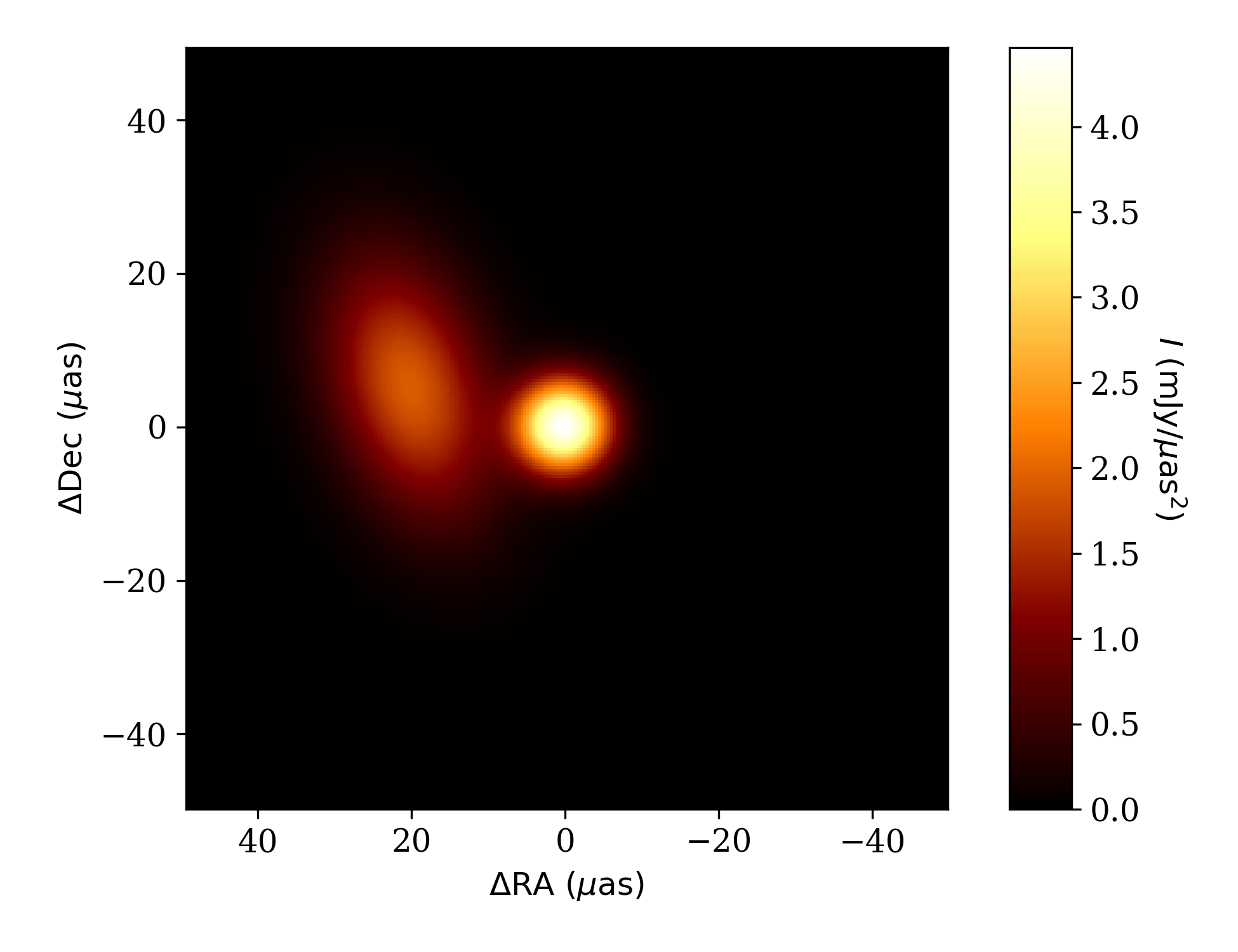
Image of the brightness map for the binary model made using the
fisher.fisher_forecast.FisherForecast.display_image() function.
We begin our science forecasts with computing the uncertainties on the fluxes
and separations of the two components. To do this we make use of the
fisher.fisher_forecast.FisherForecast.marginalized_uncertainties()
function, which computes the uncertainties for each parameter after
marginalizing over all others. We specify the observation for which to
compute the uncertainties and the indices of the parameters for which we
would like uncertainty estimates.
Sigma_obs = ffg.marginalized_uncertainties(obs,p,ilist=[0,2,6,7])
Sigma_obs2 = ffg.marginalized_uncertainties(obs2,p,ilist=[0,2,6,7])

print("Sigma's for obs:",Sigma_obs)
print("Sigma's for obs2:",Sigma_obs2)
which generates the output,
Sigma's for obs: [0.00300763 0.00600743 0.00101485 0.00205108]
Sigma's for obs2: [0.00377924 0.00753871 0.00203864 0.00333373]
From this we might conclude that the reduced array is similarly capable of constraining the fluxes of the two components (differing by about 10%-15%), but is considerably worse at constraining their relative location (though still pretty great!).
We can generate plots comparing the ability of the two arrays to constrain the
RA offsets with the
fisher.fisher_forecast.FisherForecast.plot_1d_forecast() function. We
must select the observations to include (i.e., the \((u,v)\)-coverage), the
index of the parameter that we wish to plot (the RA offset is the seventh
parameter, and therefore index 6 due to the zero-offset indexing), and may
optionally set some clarifying labels to indicate which observation details the
two different curves correspond.
ffg.plot_1d_forecast([obs2,obs],p,6,labels=['ngEHT','Reduced ngEHT'])
plt.savefig('tutorial_1d.png',dpi=300)
Note that we have ensured that the typically more constraining case is plotted second by setting the order of the observations in the list.
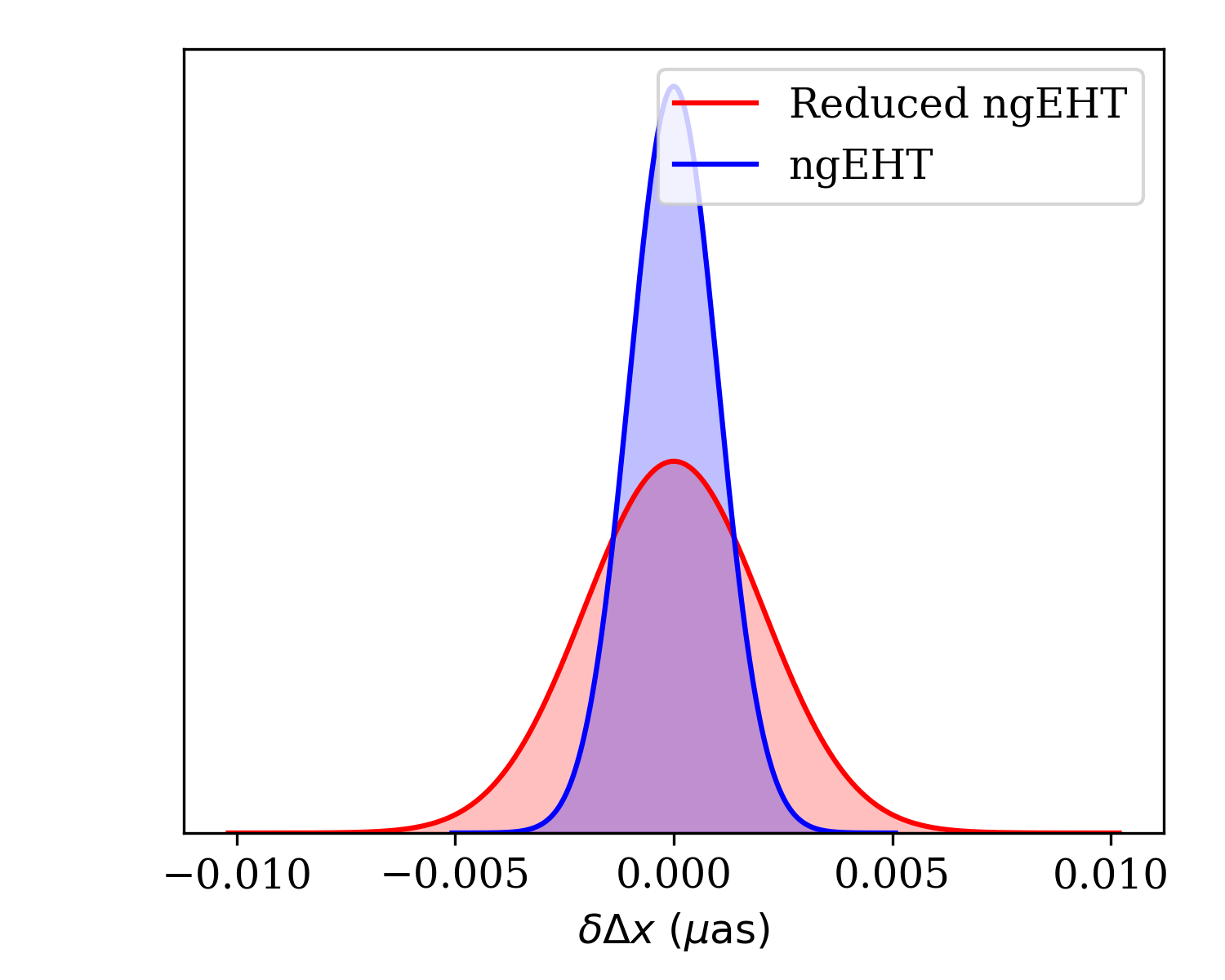
Marginalized posterior on the shift in RA between the two binary components
made using fisher.fisher_forecast.FisherForecast.plot_1d_forecast()
function. The two plots correspond to the different observations generated
in Creating an Obsdata object.
Similarly, we can generate plots of the two-dimensional joint posterior,
marginalized over all other parameters using the
fisher.fisher_forecast.FisherForecast.plot_2d_forecast() function. The
syntax is very similar to the
fisher.fisher_forecast.FisherForecast.plot_1d_forecast() function, with
the exception that now we must specify two parameter indices.
ffg.plot_2d_forecast([obs2,obs],p,6,7,labels=['ngEHT','Reduced ngEHT'])
plt.savefig('tutorial_2d.png',dpi=300)
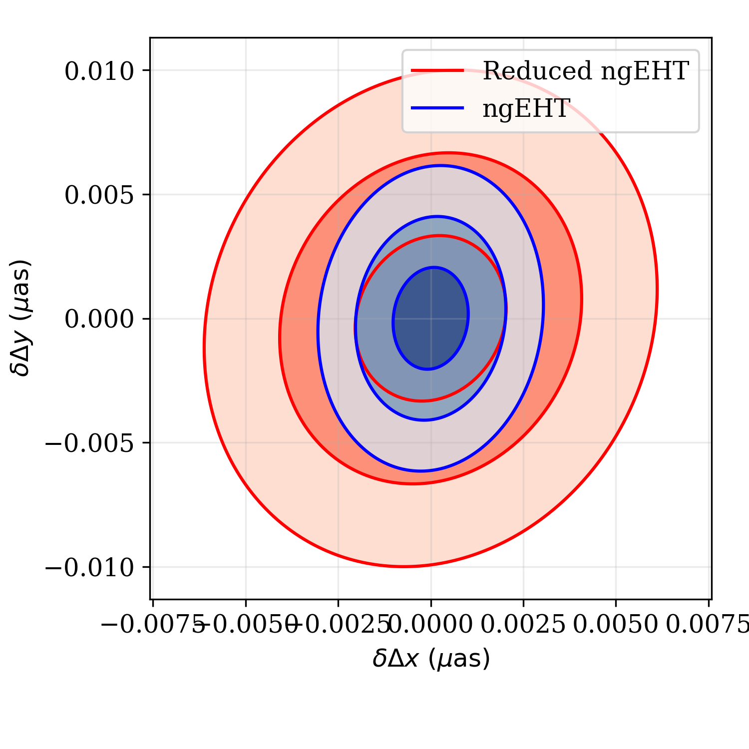
Marginalized joint posterior on the shift in RA and Dec between the two
binary components made using
fisher.fisher_forecast.FisherForecast.plot_2d_forecast()
function. The two sets of contours correspond to the different observations
generated in Creating an Obsdata object.
A triangle plot, which is simply a collection of marginalized joint and
one-dimesional posteriors, may be generated via the
fisher.fisher_forecast.FisherForecast.plot_triangle_forecast() function.
Again, the syntax is very similar, the only difference being the manner in which
indices are specified. By default, all parameters are included. It is helpful
to also include some guidance on the location relative to the figure to ensure
labels are visible.
ffg.plot_triangle_forecast([obs2,obs],p,labels=['ngEHT','Reduced ngEHT'],axis_location=[0.075,0.075,0.9,0.9])
plt.savefig('tutorial_tri.png',dpi=300)
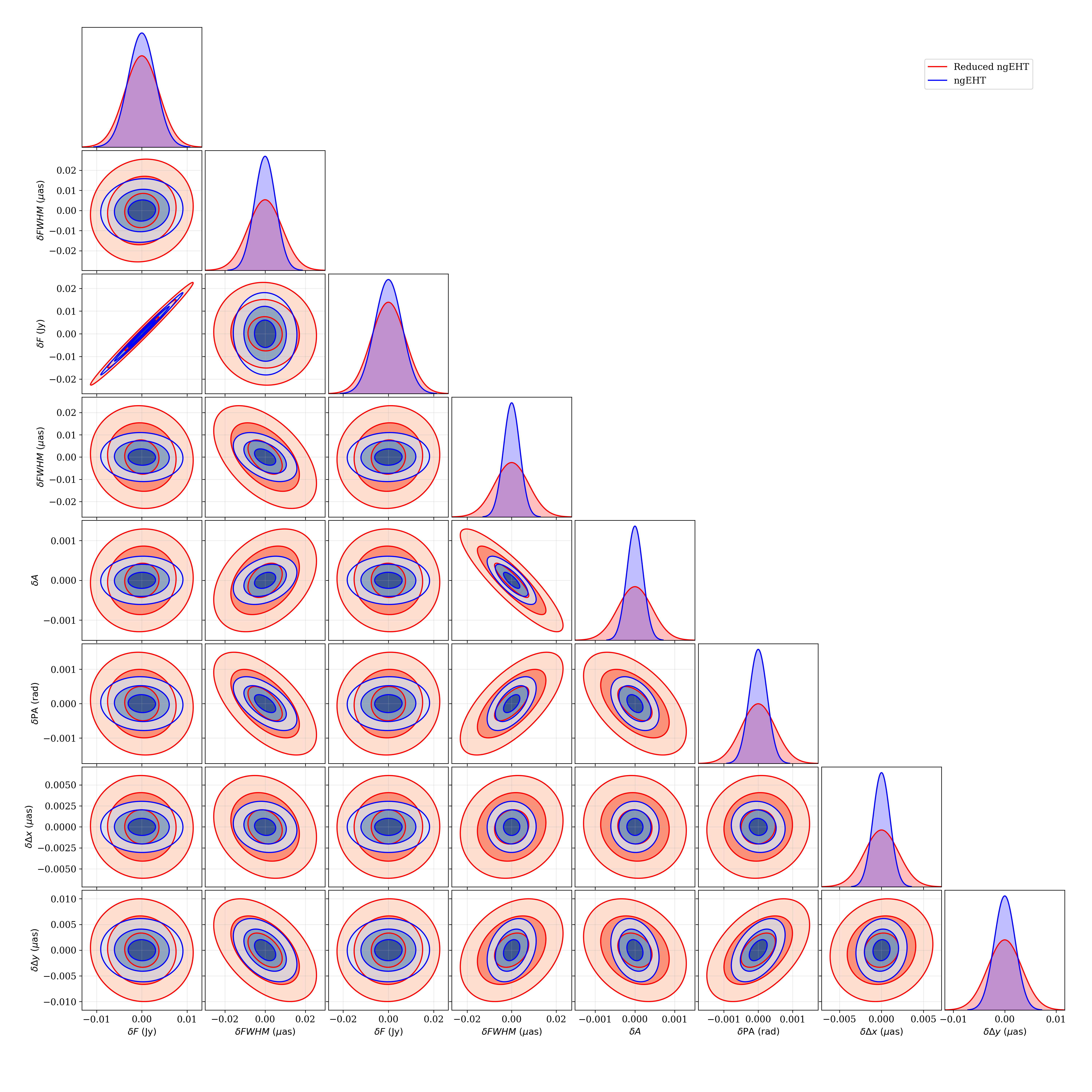
Triangle plot for the binary model made using
fisher.fisher_forecast.FisherForecast.plot_triangle_forecast()
function. The two sets of contours correspond to the different observations
generated in Creating an Obsdata object.
Chains of samples of the posterior forecasts can be produced via the
fisher.fisher_forecast.FisherForecast.sample_posterior() function.
These chains can be generated for a subset of the parameter space, marginalizing
the posterior analytically over the remaining parameters. For example, to add
samples to the joint parameter plot made above:
chain = ffg.sample_posterior(obs,p,100,ilist=[6,7])
ffg.plot_2d_forecast([obs2,obs],p,6,7,labels=['ngEHT','Reduced ngEHT'])
plt.plot(chain[:,0],chain[:,1],'.b')
plt.savefig('tutorial_2d_wsamples.png',dpi=300)
Chains can be used to assess the implications for quantities that are functions of the underlying model parameters in a fashion similar to those employed in typical sampling methods. While for many such cases, applying standard error propagation formulae will be more efficient, when the function is complicated or nonlinear, sampling can be conceptually more simple and practically more useful.
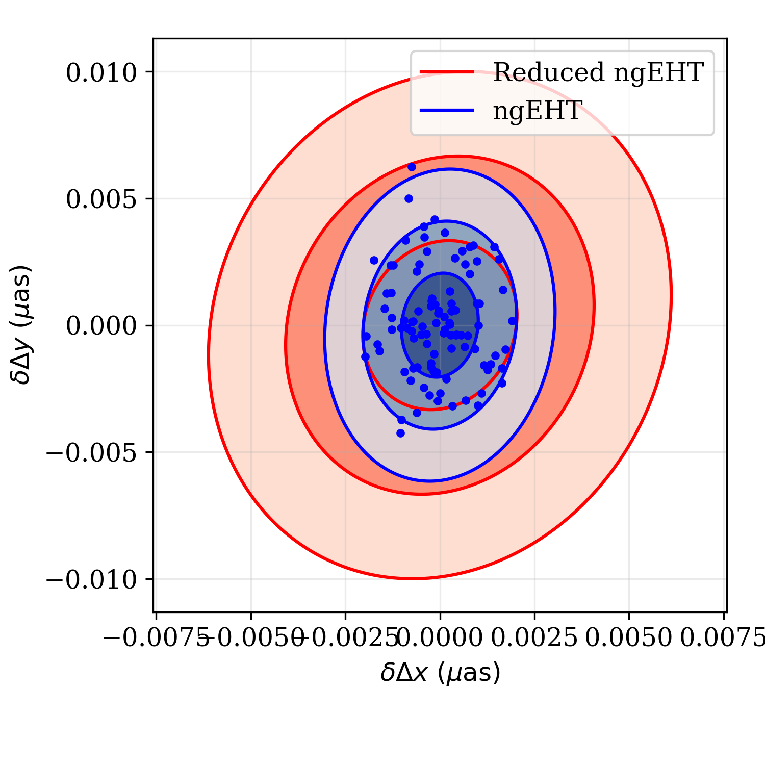
Marginalized joint posterior on the shift in RA and Dec between the two
binary components made using
fisher.fisher_forecast.FisherForecast.plot_2d_forecast()
function together with 100 samples drawn from the “ngEHT” posterior using
the fisher.fisher_forecast.FisherForecast.sample_posterior().
All of the above may be found in the Python script tutorials/forecasting.py.
Splined Raster Models
A splined-raster model, i.e., “themage”, is available in the
fisher.ff_models.FF_splined_raster class. This provides a flexible image
model that can assess imaging performance and hybrid imaging-modeling
performance. However, the large number of parameters can make it difficult to
sensibly specify an image. Therefore, a number of special ways to construct a
parameter list are available.
In this tutorial we will construct a splined-raster model and initialize it
using an existing FisherForecast object, the name of a FisherForecast child
class, a FITS file, and an ehtim.image.Image object.
We begin by constructing a splined-raster model. At initialization, we must specify the size of the raster, i.e., the number of control points in each direction, and the field of view of the raster. In this case, we choose 20 control points in each direction and a field of view of 60 uas:
import ngEHTforecast.fisher as fp

ff = fp.FF_splined_raster(20,60.0)
This model has 400 control points, and thus 400 parameters: the log of the
intensities at each control point. Even if the intensity is well defined,
initializing 400 parameters is a daunting task! Fortunately, a number of
options are available with the
fisher.ff_models.FF_splined_raster.generate_parameter_list() function.
The first we consider is initializing from an existing FisherForecast object. We
begin by creating another
fisher.ff_models.FF_smoothed_delta_ring object. This is then passed to
the fisher.ff_models.FF_splined_raster.generate_parameter_list() function
along with the parameter list (here for a total flux of 1 Jy, diameter of 40 uas,
and width of 10 uas) as a key-word argument. We pass an additional argument,
limits, which specifies the extent of the image created by the
fisher.fisher_forecast.display_image() function.
ffinit = fp.FF_smoothed_delta_ring()
pinit = [1.0, 40.0, 10.0]

p = ff.generate_parameter_list(ffinit,p=pinit,limits=100)
To compare the in splined-raster model and original smoothed delta-ring, we display both:
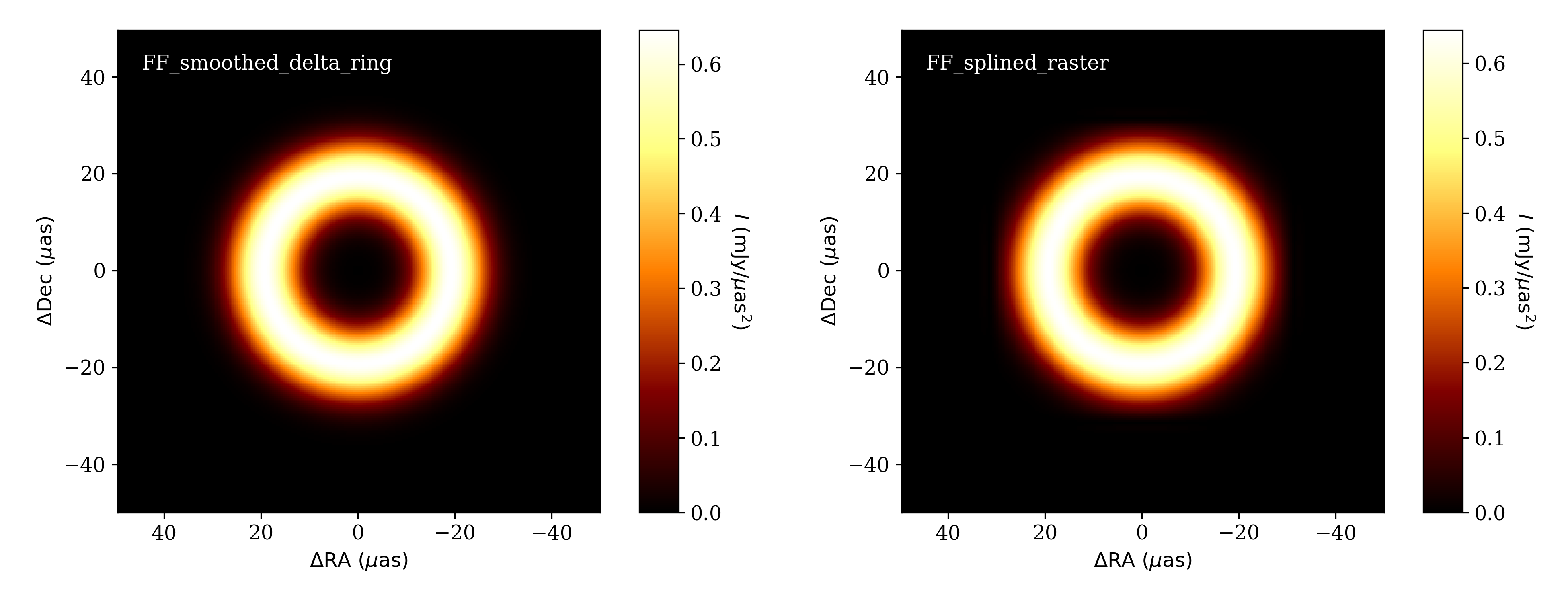
Smoothed delta-ring model (left) and the splined raster model initialized from it (right).
The second is an initialization from a FisherForecast model without actually constructing an instantiation. This avoids the overhead of creating the model, but still leverages the other FisherForecast models. In this case, we use an asymmetric Gaussian model with total flux 1 Jy, symmerized FWHM of 20 uas, asymmetry parameter of 0.5, and PA of 1.0 rad:
p = ff.generate_parameter_list(fp.FF_asymmetric_gaussian,p=[1,20,0.5,1.0])
In the third example, we initialize from an ehtim.image.Image object,
which we create from a FITS file.
import ehtim as eh

img = eh.image.load_fits('M87_230GHz.fits')
img = img.blur_circ(np.sqrt(ff.dxcp*ff.dycp))

p = ff.generate_parameter_list(img)
Prior to generating the splined raster parameter list, we blur the image to the raster resolution to give a better impression of the results of a splined raster fit. The result is shown below.
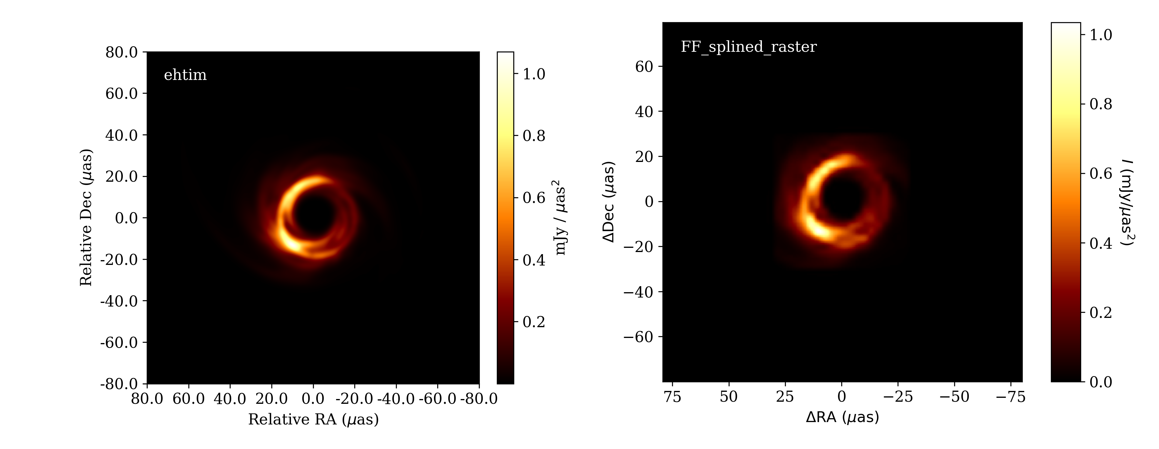
Image from ehtim (left) and the splined raster model initialized from it (right).
Finally, we can initialize the parameter list from a FITS file directly. This
is identical to initializing from an ehtim.image.Image object, which it
creates internally, including blurring to the raster resolution.
p = ff.generate_parameter_list('M87_230GHz.fits')
All of the above may be found in the Python script tutorials/splined_raster_initialization.py.
Data Preprocessing
While data generation lies outside the scope of ngEHTforecast, some data
processing steps are most conveniently handled within ngEHTforecast. For
example, detection thresholds depend on the source structure, and therefore
cannot be applied until a FisherForecast model and parameter set are chosen. The
function data.processing.process_obsdata() exists to faciliate minor
preprocessing steps, including those that depend on the particular model
selected.
In this tutorial, we will review the features of
data.processing.process_obsdata() and how to use them to average the data,
model detection thresholds, and add various systematic components to the
uncertainties on the complex visibilities.
Given either a preexisting ehtim.obsdata.Obsdata object or a UVFITS
file name, we can begin. Without additional options,
import ngEHTforecast.data as fd

obs = fd.preprocess('../uvfits/M87_230GHz.uvfits')
returns the Obsdata object constructed by the ehtim.obsdata.load_uvfits()
function.
Averaging the data over scans increases the SNR of individual data points and reduces data volume. To perform this averaging,
obs = fd.preprocess('../uvfits/M87_230GHz.uvfits',avg_time='scan')
Alternatively, a scan period can be specified in seconds.
Applying a detection threshold should follow the definition of a FisherForecast object, which we take in this example to be a symmetric Gaussian with a total flux of 1 Jy and FWHM of 40 uas:
import ngEHTforecast.fisher as fp
ff = fp.FF_symmetric_gaussian()
p = [0.6,40]

obs = fd.preprocess('../uvfits/M87_230GHz.uvfits',avg_time='scan',ff=ff,p=p,snr_cut=10)
where we have removed all data points that have an SNR below 10 after setting the complex visibilities using the symmetric Gaussian model and scan averaging. Note that this step will depend on the particular model adopted and parameter values chosen.
Non-closing systematic errors are typically incorporated via an additional fractional error, and is most sensibly applied after specifying a FisherForecast object. A constant error floor, like that used to mitigate scattering in the Galactic center, may be specified independent of the underlying model. Therefore, to add an additional 2% fractional error and 10 mJy error floor:
obs = fd.preprocess('../uvfits/M87_230GHz.uvfits',sys_err=2,const_err=10.0,ff=ff,p=p)
To explore the data at any point, a handful of functions are provided to display the data sets. The baselines and visibilities can be plotted:
display_visibilities(obs)
display_baselines(obs)
Multiple data sets can be overplotted by use of the fig and axs/axes options. For example, to plot the \((u,v)\)-coverage for different data sets, we could do the following:
_,ax = fd.display_baselines(obs1)
fd.display_baselines(obs2,axes=ax,color='r')
Which generates the baseline map:
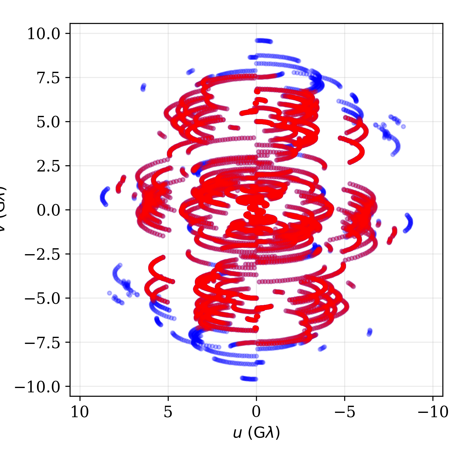
Baseline map of two data sets with different SNR cuts generated with the
data.processing.display_baselines() function.
Similarly, we can combine different visibility plots:
_,axs = fd.display_baselines(obs1)
fd.display_baselines(obs2,axes=axs,color='r')
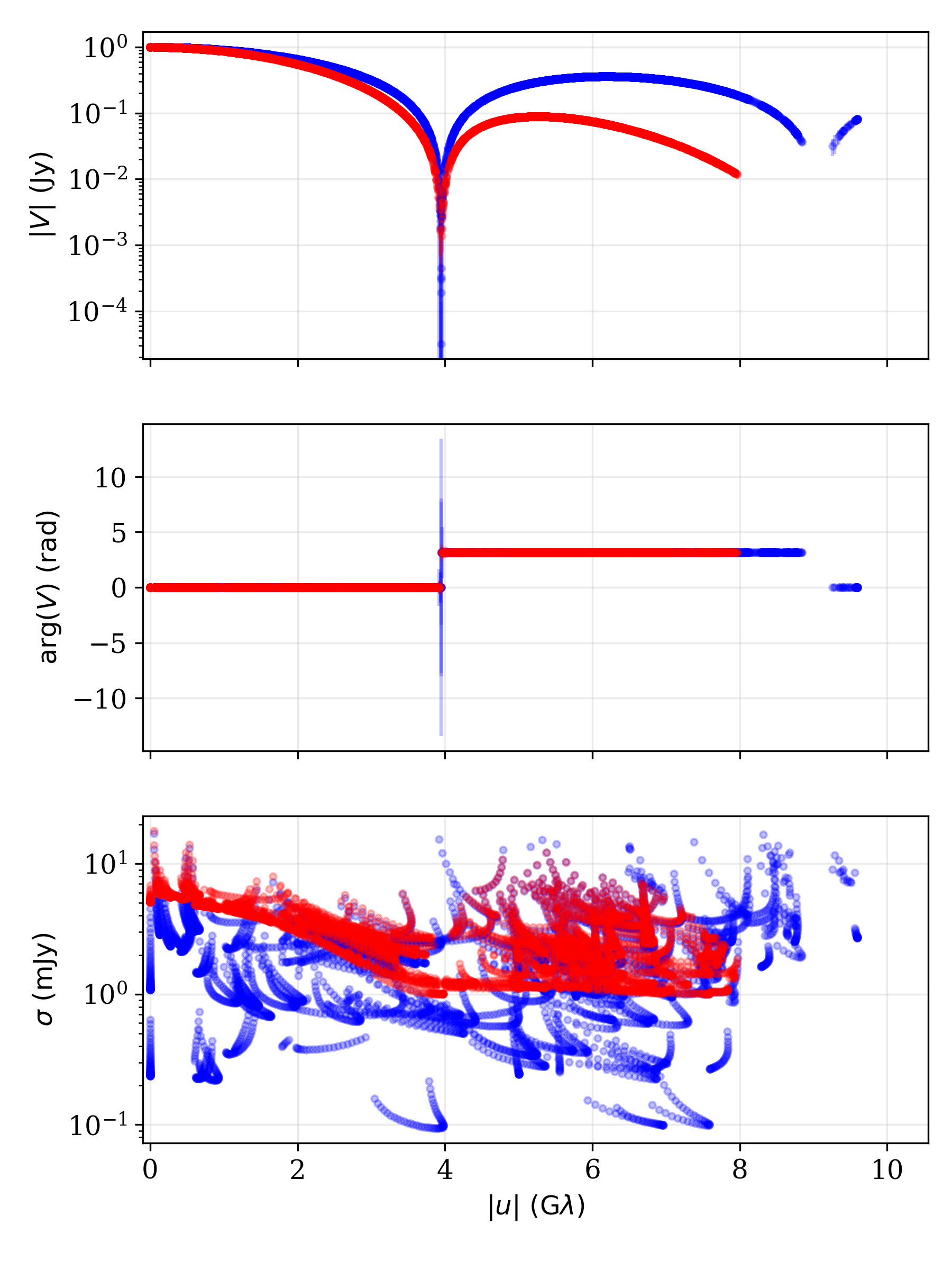
Data summary plot of two data sets showing the complex visibilities and
uncertainties generated with the data.processing.display_visibilities()
function.
A minimal data quality assessment can be obtained by looking at closure phases on trivial triangles. In principle, these should identically vanish, though may deviate from zero by an amount that depends on how short the degenerate baseline is and the degree of extended structure. Nevertheless, these closure phases provide a simple test of the internal consistency of the data. The trivial closure phases may be identified and displayed via
fd.display_trivial_cphases(obs,print_outliers=True)
which plots the values of the trivial closure phases and the distribution of the normalized residuals. If outlying cases are found, they will be printed in the above example. The result is:
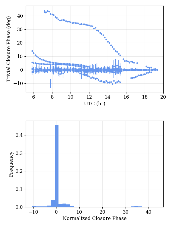
Trivial closure phases and their normalized residual distribution, generated
with data.processing.display_trivial_cphases() function.
179 2-sigma outliers found.  Printing only worst 20.
[(10.66666675, 'ALMA', 'APEX', 'LMT', 319021.84375   , -1524516.375, 2.41010099e+09, -3.68364518e+09, -2.17140198e+09, 3.31984947e+09, 34.69365821, 0.39219712)
 (10.83333349, 'ALMA', 'APEX', 'LMT', 285234.75      , -1521679.375, 2.42862182e+09, -3.66092698e+09, -2.18805197e+09, 3.29938150e+09, 34.49958923, 0.39019933)
 (10.5       , 'ALMA', 'APEX', 'LMT', 352198.375     , -1527667.875, 2.38696730e+09, -3.70616781e+09, -2.15059558e+09, 3.34014157e+09, 34.76051541, 0.39505022)
 (11.16666698, 'ALMA', 'APEX', 'LMT', 216088.453125  , -1516969.625, 2.45169178e+09, -3.61507840e+09, -2.20876493e+09, 3.25807514e+09, 34.02358379, 0.38889065)
 (10.33333325, 'ALMA', 'APEX', 'LMT', 384700.75      , -1531127.625, 2.35926502e+09, -3.72845158e+09, -2.12567296e+09, 3.36021888e+09, 34.8401166 , 0.39883577)
 (11.49999976, 'ALMA', 'APEX', 'LMT', 145288.578125  , -1513574.625, 2.45600051e+09, -3.56897229e+09, -2.21257574e+09, 3.21653837e+09, 33.9200136 , 0.38831674)
 (11.00000024, 'ALMA', 'APEX', 'LMT', 250901.71875   , -1519162.125, 2.44249421e+09, -3.63805670e+09, -2.20051430e+09, 3.27877709e+09, 33.87802113, 0.39004852)
 (11.33333302, 'ALMA', 'APEX', 'LMT', 180861.609375  , -1515105.875, 2.45619686e+09, -3.59203558e+09, -2.21278771e+09, 3.23731558e+09, 33.77896262, 0.38892976)
 ( 9.83333302, 'ALMA', 'APEX', 'LMT', 477548.34375   , -1543288.   , 2.24931968e+09, -3.79344742e+09, -2.02672410e+09, 3.41878093e+09, 35.82138766, 0.41379818)
 ( 9.99999976, 'ALMA', 'APEX', 'LMT', 447435.8125    , -1538945.25 , 2.29037517e+09, -3.77213338e+09, -2.06367808e+09, 3.39957632e+09, 35.28836523, 0.40826177)
 (10.16666651, 'ALMA', 'APEX', 'LMT', 416466.84375   , -1534889.125, 2.32704717e+09, -3.75045402e+09, -2.09668224e+09, 3.38004301e+09, 34.71594624, 0.40391181)
 (11.66666651, 'ALMA', 'APEX', 'LMT', 109437.484375  , -1512378.625, 2.45110374e+09, -3.54593357e+09, -2.20812851e+09, 3.19578291e+09, 33.29811963, 0.38943998)
 (11.83333325, 'ALMA', 'APEX', 'LMT',  73376.921875  , -1511520.375, 2.44151526e+09, -3.52296192e+09, -2.19945498e+09, 3.17508915e+09, 33.15342344, 0.39005985)
 ( 9.66666698, 'ALMA', 'APEX', 'LMT', 506746.875     , -1547909.375, 2.20395878e+09, -3.81435597e+09, -1.98589107e+09, 3.43762022e+09, 35.83029137, 0.42265596)
 (12.        , 'ALMA', 'APEX', 'LMT',  37175.91015625, -1511001.25 , 2.42725402e+09, -3.50010317e+09, -2.18657178e+09, 3.15449626e+09, 33.01515858, 0.39076589)
 ( 9.50000024, 'ALMA', 'APEX', 'LMT', 534975.5625    , -1552800.375, 2.15437952e+09, -3.83481830e+09, -1.94125709e+09, 3.45605862e+09, 36.09585198, 0.43218905)
 ( 9.33333349, 'ALMA', 'APEX', 'LMT', 562180.25      , -1557951.625, 2.10067699e+09, -3.85479629e+09, -1.89290752e+09, 3.47406029e+09, 36.83603985, 0.44147205)
 (12.16666603, 'ALMA', 'APEX', 'LMT',    903.74713135, -1510822.5  , 2.40834662e+09, -3.47739955e+09, -2.16950349e+09, 3.13404416e+09, 32.55422891, 0.39210264)
 (12.33333349, 'ALMA', 'APEX', 'LMT', -39264.10546875, -1677331.125, 2.38483021e+09, -3.45489510e+09, -2.14828262e+09, 3.11377203e+09, 32.22049294, 0.39305758)
 ( 9.16666675, 'ALMA', 'APEX', 'LMT', 588308.9375    , -1563353.125, 2.04295360e+09, -3.87425101e+09, -1.84093491e+09, 3.49159091e+09, 36.91539343, 0.45524961)]
  ...
-------------------------------------------------------------------
Examples of the above may be found in the Python script tutorials/data_preproc.py.
Data Generation
Simulated data sets can be generated from
fisher.fisher_forecast.FisherForecast objects using the with ngehtsim
package. While examples exist within the ngehtsim repository, here we review
some basic functionality, though see the ngehtsim documentation for detailed
information.
We begin by importing the ngehtsim observation generation functionality. This presumes that ngehtsim is installed (see the ngehtsim documentation).
import ngehtsim.obs.obs_generator as og
import ngEHTforecast as nf
import matplotlib.pyplot as plt
We then construct a fisher.fisher_forecast.FisherForecast object and
set of parameters from which visibilities will be constructed:
ff = nf.fisher.FF_symmetric_gaussian()
p = [0.05,20.0]
We then specify various setting options for the observation generator. Reasonable defaults exist for each setting, and these may be specified separately in a state file (see the ngehtsim documentation). A subset of potential options are listed here, including setting the weather profile (here ‘poor’), source name, source position, observation frequency, and array choice.
settings = {}
settings['weather'] = 'poor'
settings['source'] = 'Test'
settings['RA'] = 12.4852 # 12h 29m 06.7s
settings['DEC'] = 2.0525 # +02° 03′ 09″
settings['frequency'] = '230' # GHz
settings['array'] = 'ngEHTphase1'
An ngehtsim obs.obs_generator.obs_generator object is created and an
observation generated, packaged as an ehtim.obsdata.Obsdata object.
obsgen = og.obs_generator(settings)
obs_poor = obsgen.make_obs(ff,p=p,addnoise=False,addgains=False)
Note that we have turned off the additions of noise and gains as we are interested in typical array performance. However, neither is manditory. We make a second data set after modifying the settings, in this instance changing the weather:
settings['weather'] = 'good'
obsgen = og.obs_generator(settings)
obs_good = obsgen.make_obs(ff,p=p,addnoise=False,addgains=False)
The two data sets, [obs_good, obs_poor], are now available for making science forecasts. We use the ngEHTforecast data visualization to look at the data and then generate a triangle plot of the two generated data sets:
_,ax = nf.data.display_baselines(obs_good,color='b')
nf.data.display_baselines(obs_poor,axes=ax,color='r')
plt.savefig('ngehtsim_uv.png',dpi=300)

_,axs = nf.data.display_visibilities(obs_good,color='b')
nf.data.display_visibilities(obs_poor,axs=axs,color='r')
plt.savefig('ngehtsim_vis.png',dpi=300)

ff.plot_triangle_forecast([obs_good,obs_poor],p,axis_location=[0.2,0.2,0.75,0.75],labels=[r'Good weather',r'Poor weather'])
plt.savefig('ngehtsim_tri.png',dpi=300)
which generates the following plots:
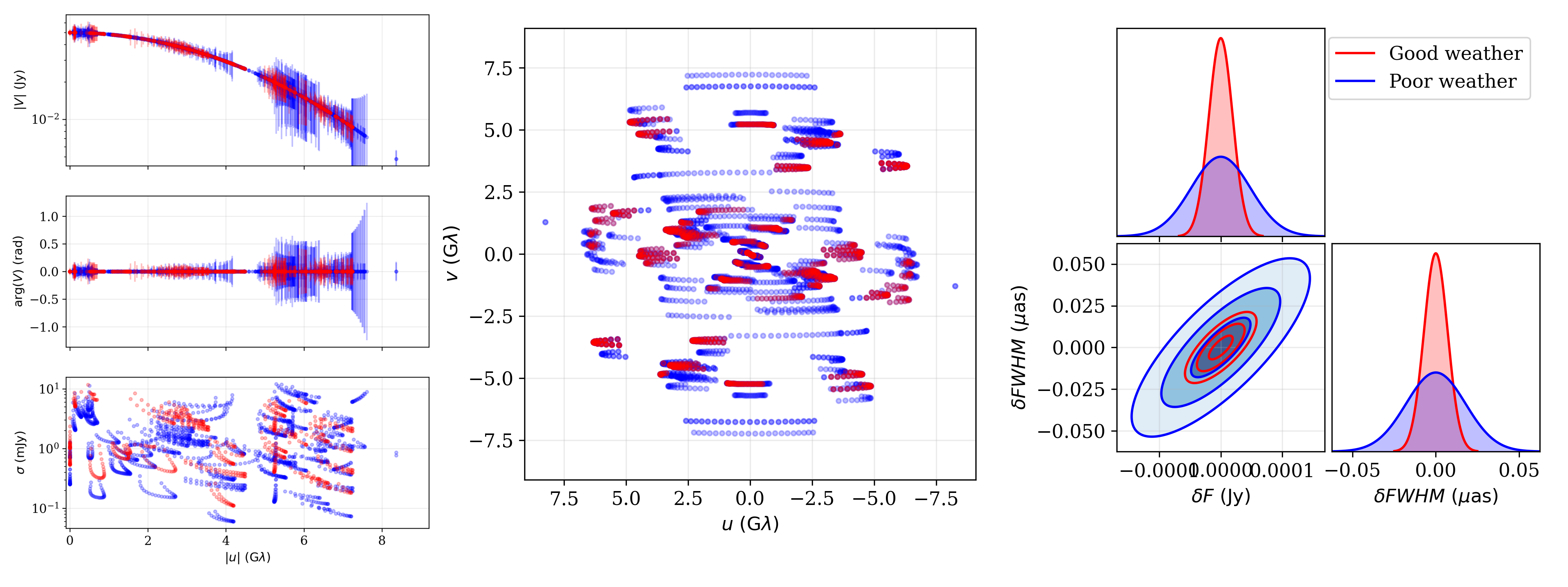
Visibilities and uncertainties (left), baseline map (center), and joing posterior (right) for the good and poor weather data sets.
Examples of the above may be found in the Python script tutorials/ngehtsim_example.py.
Exploring & Parallelization
A key question for many science cases will be how the uncertainties depends on specific model prameters. For example, how well the binary separation can be determined as a function of the flux of the secondary. In this tutorial, we will make a plot that shows how a chosen parameter uncertainty varies with respect to the source model parameters. Because large parameter space explorations can quickly become computationally intensive, we will also demonstrate how this can be parallelized to take advantage of multiple cores.
Exploring parameter dependence can easily addressed via an appropriate loop over
the model paramters. Again, we will assume that the code from the tutorials
Creating an Obsdata object and Creating a FisherForecast object is
included. The only ngEHTforecast function that we are using is the same
fisher.fisher_forecast.FisherForecast.marginalized_uncertainties()
described in Forecasting Uncertainties. However, now it is embedded
in a loop which varies the “truth” parameters:
secondary_flux = np.logspace(-3,0,16)
Sigma_list = 0*secondary_flux
for i in range(len(secondary_flux)) :
    p = [0.5,10, secondary_flux[i],20,0.5,0.3, 20,5]
    Sigma_list[i] = ffg.marginalized_uncertainties(obs,p,ilist=6)

import matplotlib.pyplot as plt

plt.plot(secondary_flux,Sigma_list,'-ob')
plt.xscale('log')
plt.yscale('log')
plt.xlabel(r'Flux of Secondary (Jy)')
plt.ylabel(r'$\sigma_{\rm RA}~(\mu{\rm as})$')
plt.grid(True,alpha=0.25)

plt.savefig('tutorial_sep',dpi=300)
The remainder of the code makes a Matplotlib plot, specifies the scales, adds labels and other accoutrements, and saves the following plot to a file.
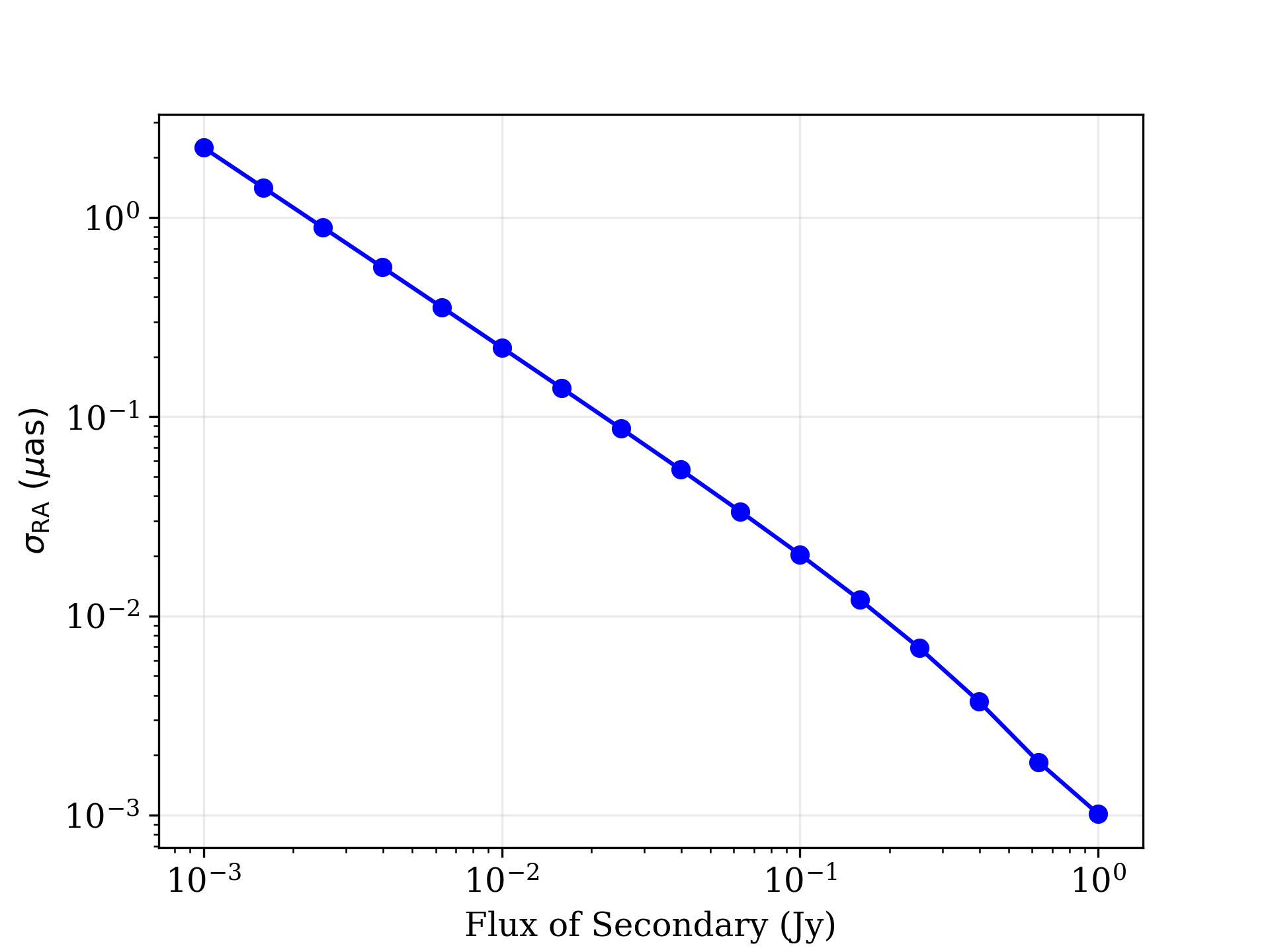
Uncertainty on the separation in RA as a function of the total flux of the secondary in the binary model.
All of the above may be found in the Python script tutorials/binary_separation.py.
While the above code completes in approximately 1 minute on a single modern core, increasing the number of parameters being surveyed rapidly grows the computational expense. Beacause the loop is trivially parallel, the evaluation of the uncertainty at each parameter set is independent of all others, this problem lends itself to parallelization.
There are many packages that enable parallelization in Python. We will make use of two: the the Joblib package and multiprocessing library. We begin with the former, Joblib.
All that changes from above is the syntax surrounding the computation of the
elements of Sigma_list. From Joblib we import the functions
joblib.parallel.Parallel and joblib.parallel.delayed() (see the Joblib
documentation for why the latter is useful). Joblib will handle the
distribution of individual computations to the cores (here set to 4), we must
only define a single function to return the desired marginalized uncertainty at
each new point in the parameter space.
from joblib import Parallel, delayed

def get_sigma(flux) :
    p = [0.5,10, flux,20,0.5,0.3, 20,5]
    return ffg.marginalized_uncertainties(obs,p,ilist=6)

secondary_flux = np.logspace(-3,0,16)
Sigma_list = Parallel(n_jobs=4)(delayed(get_sigma)(flux) for flux in secondary_flux)

import matplotlib.pyplot as plt
...
plt.savefig('tutorial_sep_joblib.png',dpi=300)
We do so by defining a small function that, when given a flux for the secondary,
sets the parameter list and returns the marginalized uncertaint on the RA
offset. This function is then passed to joblib.parallel.Parallel using
joblib.parallel.delayed() as specified in the Joblib documentation.
The advantage of using Joblib is that the entirety of the modification due to parallelization is to define as a function the elements of the computation that we wish to parallelize and some minor syntax changes. This version of the binary separation may be found in the Python script tutorials/binary_separation_joblib.py.
Alternatively, we can make use of the Python multiprocessing library. Again, the primary difference is that part we wish to parallelize is most conveniently contained in a single function. To parallelize across 4 processes:
import multiprocessing as mp

def get_sigma(flux) :
    p = [0.5,10, flux,20,0.5,0.3, 20,5]
    return ffg.marginalized_uncertainties(obs,p,ilist=6)

if __name__ == "__main__" :
    secondary_flux = np.logspace(-3,0,16)

    with mp.Pool(4) as mpp :
        Sigma_list = mpp.map(get_sigma,secondary_flux)

    plt.plot(secondary_flux,Sigma_list,'-ob')
    ...
    plt.savefig('tutorial_sep_multiproc.png',dpi=300)
To avoid repeating the initialization steps (loading the UVFITS file, creating
the fisher.fisher_forecast.FisherForecast), per the multiprocessing
library documentation, the portion of the code that will ultimately be
parallelized is contained in the __name__ == “__main__” guards. This version
of the binary separation may be found in the Python script
tutorials/binary_separation_multiprocessing.py.